The integration time is the time a sensor on a microplate reader spends to collect and accumulate light or a signal. If the intensity of the emission signal is plotted against the integration time at the detector, then the area under the curve for a specific time window represents the intensity of the emission signal.
BMG LABTECH microplate readers are equipped with photomultiplier tubes (PMTs) to detect emission signals. At the PMT, the integration time refers to the time that the PMT collects photons that are subsequently converted to an electrical signal. The integration time can have a significant influence on the quality of the data. Optimising the integration time is especially relevant in the detection of signals with an extended decay time like luminescence, time-resolved fluorescence and AlphaScreen®.
Did you know?
On BMG LABTECH microplate readers you can select integration times between 0.01 and 100 s when measuring luminescence. The signal can be normalised to 1s to compare different measurements.
Integration time in luminescence measurements
In luminescence, photons arise due to a chemiluminescent event from a substrate in an electronically excited state. If the signal is detected over a longer interval of time, more photons can reach the PMT (fig. 1A) and the signal increases with the interval time (fig. 1B). There are essentially no restrictions on the set integration time. Classic glow assays often emit light for several minutes or even hours.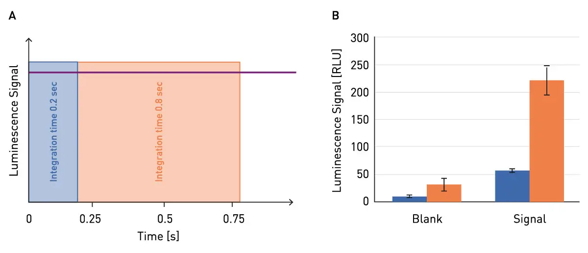
The positive effect of higher integration times on data quality is best explained with statistics. Variations in measured values occur depending on the quality
of the sample and the specifications of the measuring device. These upward or downward fluctuations are less significant the more data points are recorded and averaged per sample. This relationship is also explained in detail in our How to Note on the influence of the flash number, in the example described for fluorescence measurements. The variability of the data is reduced as the flash number increases since more measurements are included in the averaging of the final measured value. The same principle applies to the integration time. Although no average values are calculated for several different measurements, the signal is determined over a certain time by the cumulative signal resulting from the arrival of all photons in the time interval which ultimately has the same effect.
Did you know?
An assay and instrument are considered excellent when the Z´ value is between 0.5 and 1.
A comparison of the data quality from samples analysed with a glow luminescence assay using varying integration times is shown in fig. 2. The coefficient of variance (%CV) indicates the data variability. The %CV decreases when measuring the same samples at increasing integration times. Consequently, higher integration times generate more reliable and robust data (fig. 2A). Individual upward or downward fluctuations gain in importance as integration time decreases, but their impact significantly decreases with long integration times. The %CV approaches a plateau, when a solid integration time is reached. Another factor results from the overall signal height. Here, samples with a higher signal show a lower %CV than samples with a lower signal. In general, the higher the photon yield the lower the variability of the data. For this reason, the potential improvements on the data variability due to increased integration time are lower for samples at high intensity.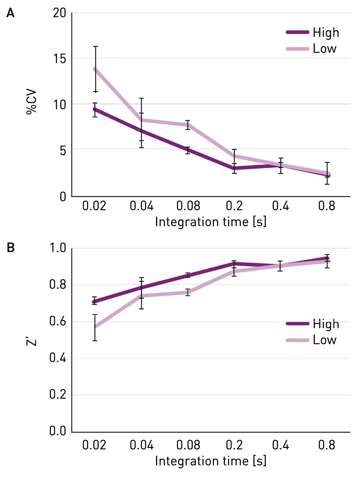
In addition to the variability of data (%CV), another statistical measure for assay quality is the Z’ value. Z’ considers the means and the standard deviations of the signals for the positive and negative controls.
In general, the higher the Z’ value, the more reliable and robust the assay results are. As shown in fig. 2B, Z’ rises with increasing integration time. This confirms a significant improvement in data quality with increasing integration time for this luminescence assay. However, if a sufficient integration time is achieved, the optimisation potential is limited. It is therefore not always necessary to use the default value for precise measurements - smaller values are usually sufficient to achieve excellent data quality. Lower integration times also significantly reduce the overall measurement time. Another reason that argues against the use of very high integration times is, background noise. Background noise may also increase disproportionately as integration time increases. Therefore, the need for higher integration times should be carefully considered and used only if necessary.
The optimisation of the integration time of measurements based on Alpha Technology will not be covered in detail in this HowToNote. In general, however, it can be based on the optimisation of luminescence measurements.
Did you know?
There are also differences in the decay of
fluorophores with a long emission. The lanthanide europium, for example, shows a significantly longer emission decay than terbium.
Integration time in time-resolved fluorescence measurements
Fluorescence arises due to the emission of light at a specific wavelength after the excitation of a fluorophore. Regular fluorophores show a very fast emission decay in the nanosecond range (fig. 3, grey curve). The excitation and detection happen almost at the same time for short-lived fluorescence. For fluorophores like lanthanides with long emission times, detection can be prolonged to the micro- or even millisecond range. Here, the integration time can be extended or the measurement time delayed without the signal falling to levels that cannot be reliably detected. This is called time-resolved fluorescence (TRF; fig. 3, purple curve).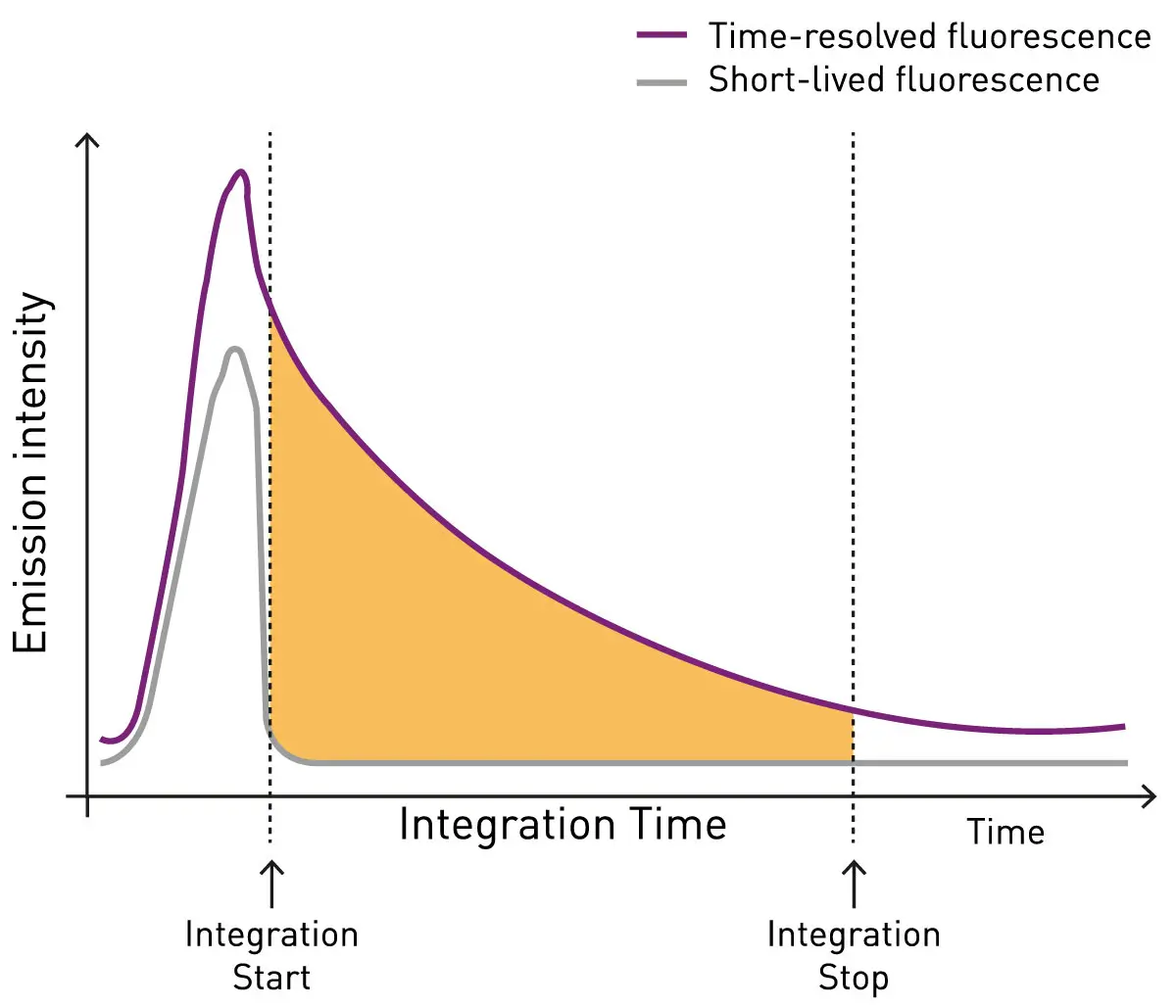
Did you know?
BMG LABTECH microplate readers are equipped with photomultiplier tubes (PMT) to detect emission signals. The PHERAstar FSX contains two pairs of matched PMTs which are used for Simultaneous Dual emission (SDE), saving time and decreasing data variability.
In Time-Resolved Förster Resonance Energy Transfer (TR-FRET), two emission signals are measured. The emission of the donor fluorophore is present upon excitation, while the acceptor emission signal depends on the interaction of donor and acceptor binding partners (fig. 4).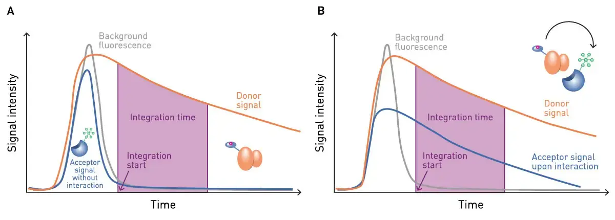
Adjustment of the integration time is also key to optimise data quality in TRF assays. In TR-FRET assays, two parameters are regularly used to monitor the performance: Delta F is used to evaluate the assay window and is also referred to as the dynamic range; Z‘ is primarily used to analyse the general data quality including data variability.
The data quality of a TR-FRET assay at different integration times is shown in fig. 5. Two standards were measured with a TR-FRET assay at different integration times. Delta F and the assay window decrease with longer integration times. Shorter integration times provide a larger assay window. This can be explained by a decrease in the signals over the integration time, thereby lowering the difference between high and low values over time, which reduces the potential range for measurements.
Z’ values on the other hand are relatively stable, provided the integration time is kept above a certain threshold (here 200 µs). Like glow luminescence, a longer integration time allows more photons to be collected, which reduces the variability of the measurement value and results in more robust data.
For TR-FRET assays, the overall longer total measurement time per plate is not the only consideration against longer integration times. Delta F also tends to favour shorter integration times - at least in this example. To achieve optimal results, a balance must be found between Delta F and Z‘, which is normally found at a medium integration time (here between 200 and 400 µs).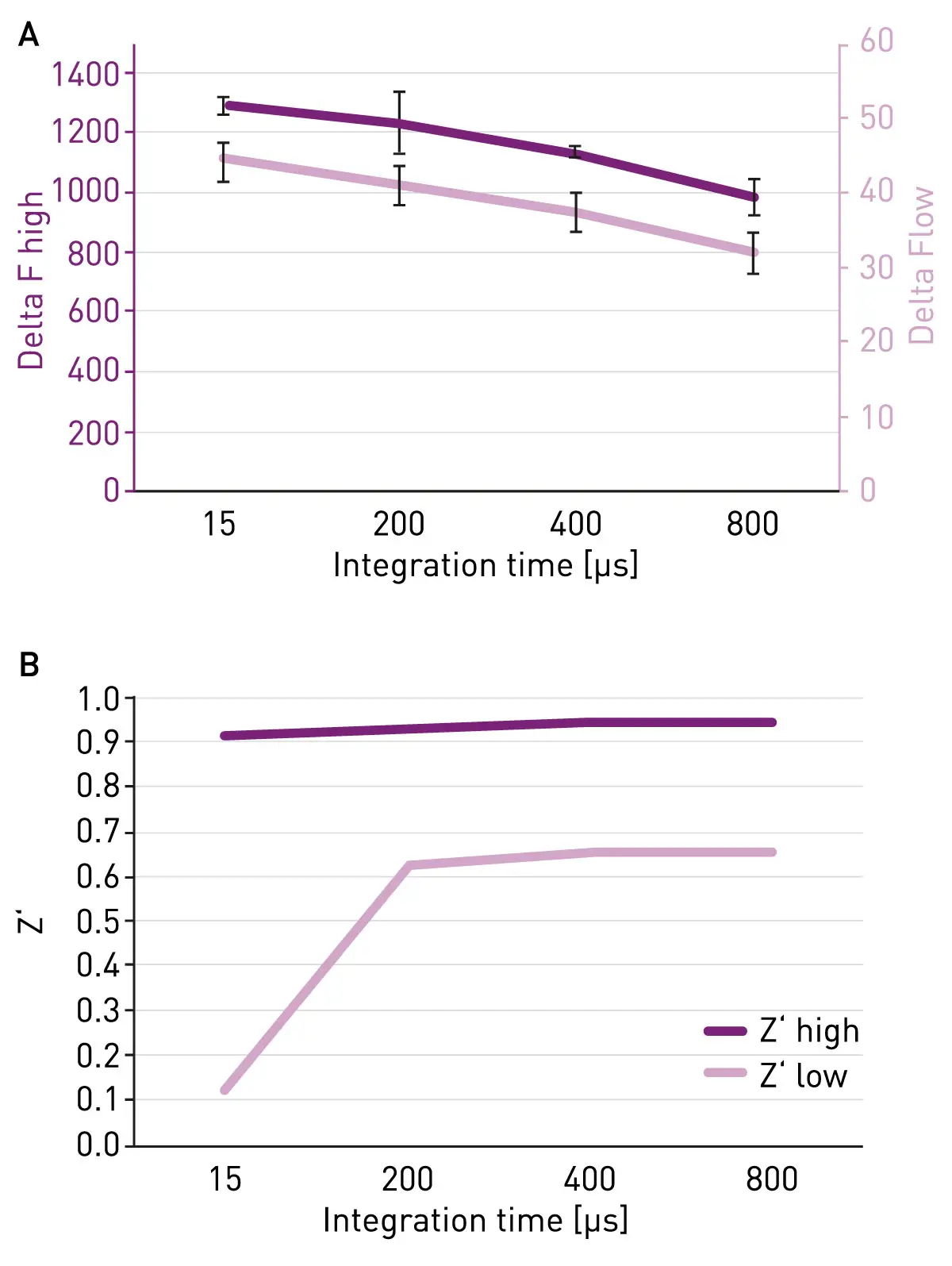
Typically, the ideal measurement settings for TR-FRET assays are provided by the manufacturer and specified in the manual of the assay kit. However, these parameters must be optimised during assay development if a commercially available kit is not used and you set up your own assays. BMG LABTECH offers a helpful tool for this on the PHERAstar® FSX: Decay Curve Monitoring. This tool saves you from having to vary the parameters manually and checking their influence on data quality individually. Here you can simply select the calculation you would like to have performed on your data (like Z’) and monitor the effects of variations in integration time and integration start time on your evaluation parameter (fig. 6). This tool not only saves you a lot of time, but it also displays the effects in a way that makes it easy to select the optimal measurement settings.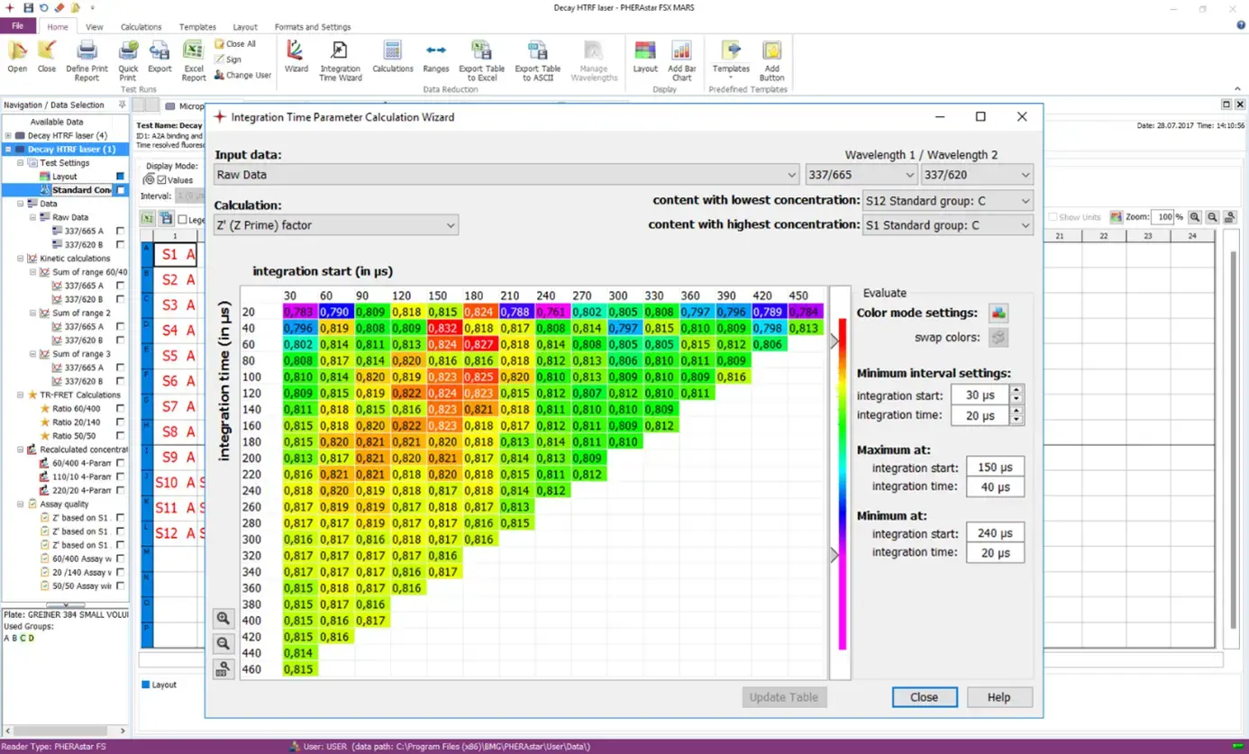
Did you know?
BMG LABTECH’s Decay Curve Monitoring feature is not only useful for TR-FRET but also for TRF and AlphaScreen® assays.
Conclusion
- Integration time affects data quality
- Longer integration times reduce data variability and increase reproducibility and robustness of measurement values
- Longer integration times may decrease the assay window and increase the total measurement time required per well and plate
- To optimise the integration time, these factors must be weighed up in each individual case
- The use of BMG LABTECH’s Decay Curve Monitoring feature is a powerful way to optimise integration timing for TRF, TR-FRET and AlphaScreen® assays
- Initial recommendation
- Detailed Recommendation